Mehr Flexibilität bei der Erstellung komplexer Gitternetze – Lose Kontaktschnittstellen jetzt für Mehrphasenströmungsmodelle verfügbar

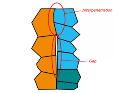
The standard interface in multi-material domain simulations is the conform mesh interface, as shown in Figure 1 left. There the first domain appears in orange color, the second in blue color. This interface is very accurate for heat transfer simulations, because each boundary face at one domain of the interface has a unique shadow boundary face. Both boundary faces have the same area, and there are no gaps or interpenetrations with the faces of the neighbor domain. All shadow boundary faces belong to the same boundary region and the same material domain. But the mesh generation with this interface is less flexible, because the whole mesh has to be created in one step.

The loose contact interface, as shown in Figure 1 right is significantly different. There, a boundary face at the interface of one domain can have several shadow boundary faces. In general the boundary faces on the first domain and the shadow boundary faces have different surface areas, and the shadow boundary faces may belong to different boundary regions and even different material domains (green domain in Figure 1 right). Gaps and interpenetrations are tolerated, and contact interfaces within the same material domain are supported. A bit lower accuracy in terms of heat transfer can be expected with such computational meshes, but there is highest flexibility in the meshing process, because each part of the mesh can be created independently from the others.

The loose contact interface functionality has been available since 2023 R2 for single-phase and since 2024 R1 for Eulerian Multiphase.

The CFD flow solver calculates the energy balance at the interfaces. For both interfaces, the standard conform and the loose contact, the heat flux is balanced in order to obtain the interface temperatures at the boundary faces. In multiphase simulation, the heat flux of the different phases, e.g. oil and vapor, and the heat release by phase change due to boiling and condensation, has to be considered additionally. The loose contact interface supports thermal resistance between the material domains leading to temperature jumps at the interface, and it has been implemented for the following multiphase models: 

• General multiphase flow without phase change (convective heat transfer only)
• General wall boiling model
• Immersion quenching model
• Jet impingement model
• RPI boiling model
• Wall condensation model

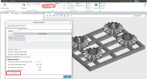
Loose contact interfaces are defined during the meshing process in AVL FAME™ , as shown in Figure 2. In the FIRE M Solver GUI no separate set-up is necessary.

The new loose contact interface for multiphase was successfully applied in an immersion quenching simulation with the general wall boiling model. The presented example is slightly changed. Oil quenching of four steel gears located on a CrMo stainless steel rack is simulated. There are three domain interfaces in the computational mesh: gears – fluid, rack – fluid, gears – rack, which are all connected by the loose contact interface. The initial temperature of the gears and the rack is 900 °C, and the initial oil and air temperatures are 20 °C. The mesh is static and the oil enters the domain from the bottom with 4 cm/s for the first six seconds in order to simulate the immersion process.

The applied general wall boiling model is a powerful model with seamless transition between film, transition and nucleate boiling regimes. Leidenfrost temperature and transitional temperature (change from nucleate boiling to transitional boiling regime) are model inputs. For oil quenching and the given initial temperature, mainly transitional and nucleate boiling can be expected. Consequently, the Leidenfrost temperature was set to a 1025 °C, which is never reached in this simulation. This ensures that the heat transfer is modelled with the transitional boiling, the nucleate boiling and the pure convection regimes. The critical heat flux factor was set to 0.3, and the transitional temperature is 525°C. Details and useful hints for model parametrization of the general wall boiling model can be found in the User Manual (see section 5.5.2.4.7.1. in FIRE M User Manual of 2024 R1). The physical time was 300 s, and the simulation is performed as Euler-Eulerian Two-Fluid simulation.

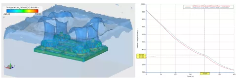
Simulation results are exemplarily shown in Figure 3. The left figure shows the solid surface temperature distribution of the gears and the rack and the iso-volume of the oil volume fraction after 10 seconds. In this initial stage of the oil quenching process the vapor formation is strong, obviously seen by the four rising vapor columns next to the gears. On the right-hand side of Figure 3 the mean temperature curves of the gears (red) and the rack (left) are shown. Since the thermal mass of the rack is higher, the cooling is slower. One can also observe a small change in the slope of the curve between 500 and 600 °C. This is the transition between transition boiling and nucleate boiling regimes. A movie of the steel quenching process in time-lapsed mode is shown in Figure 4. Note, the temperature colorbar is adjusted in each time step for better illustration. 

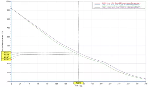
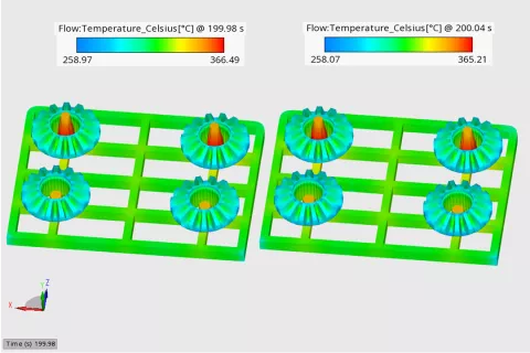
For verification, the simulation with the loose contact interface has been compared to a simulation with the standard conform mesh interface. Since the operation point and the model are the same, the simulations results have to be very similar. Figure 5 shows the comparison of the mean temperatures between gears and rack, and Figure 6 shows the comparison of the instantaneous surface temperature distributions after 200 seconds. There is perfect agreement between the two simulations. Due to the low mesh dependency of the general wall boiling model, the results are almost identical indicating that the implementation works correctly. 

Since release 2024 R1 the loose contact interfaces are available for Eulerian Multiphase in FIRE M. It is supported for all kinds of conjugate heat transfer problems in multiphase, and it correctly considers the thermal contact resistance. Loose contact is a powerful alternative to the conform multi-material interfaces. General wall boiling, RPI, wall boiling, immersion quenching, impingement quenching, and wall condensation are supported. Due to the low mesh dependency of the general wall boiling model, there is excellent agreement in the simulation results between loose contact and conform domain interfaces. The general wall boiling model of FIRE M is a unique wall boiling model which covers all relevant boiling regimes with seamless transition.