Advanced Automatic Calibration of Fuel Cells and Electrolyzers in AVL FIRE™ M
The polarization curve represents the relationship between cell voltage and current density. Achieving an accurate match between the model’s predictions and the experimental polarization curve is essential for reliable simulations. Calibration ensures that the model captures the real-world behavior of the fuel cell or electrolyzer, accounting for various losses and phenomena. Unlike simplified analytical models, CFD models operate on real-life geometries. Simplifications that do not significantly alter the polarization curve are challenging to achieve. Therefore, calibration must be performed directly on the actual geometry to account for intricate details. Even a single-cell model requires a medium to large mesh size to accurately capture flow patterns, mass transport, and electrochemical reactions. Consequently, calculating a single point on the polarization curve can take several hours due to the computational complexity. Using an optimizer on top of the fuel cell or electrolyzer model is impractical due to the lengthy calculation times. Traditional optimization techniques would significantly extend the simulation duration. An alternative approach involves calibrating parameters during the simulation run itself. As the simulation progresses, the model adjusts its parameters to match the experimental polarization curve. This dynamic calibration minimizes the need for separate optimization steps.
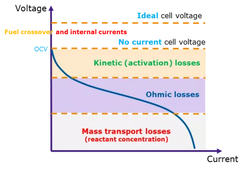
To calibrate a fuel cell model, we must analyze the typical polarization curve, see Figure 1. Performance losses observed in the curve can be attributed to specific physical phenomena:
- Fuel crossover and internal currents
- Kinetic (activation) losses: Associated with the kinetics of electrochemical reactions at the electrodes. They reflect the energy barrier that must be overcome for reactants (such as hydrogen and oxygen) to participate in the electrochemical processes.
- Ohmic losses: Arise mainly from ionic conductivity in the ionomer and electrical conductivity in the gas diffusion layers.
- Mass transport losses: Result from limitations in reactant diffusion and product removal.
In the model calibration setup of FIRE M, users have the flexibility to select the specific parameters they wish to calibrate, see Figure 2. For each performance loss, users can select a corresponding parameter to fine-tune.
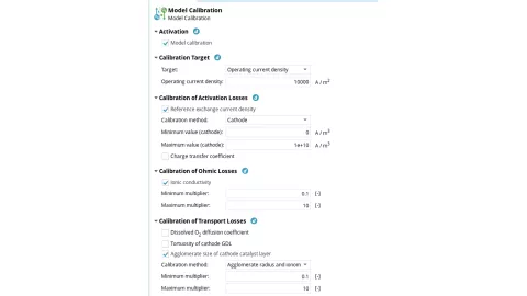
These regions cannot be adequately captured by a single operating point. Instead, for each parameter, the user must define an operating point to account for the diverse performance characteristics across the curve. These operating points are calibrated simultaneously, exchanging information about the various parameters. Prioritizing user-friendliness, the process is designed to be straightforward. Users only need to select which parameters they want to calibrate and define the same number of operating points. The critical requirement is that all operating points are calculated concurrently. The internal workings of FIRE M handle the remaining tasks. This includes making sure the right amount of parallel calculations are started, making sure different operating points are defined, coordinating parallel calculations, managing communication among different operating points, and ensuring seamless execution. Currently, interaction among the operating points occurs via the filesystem. As long as the different operating points have access to the same file system tree, they can independently perform their calculations. This approach even allows for running different operating points on separate workstations, as long as they execute simultaneously.
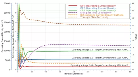
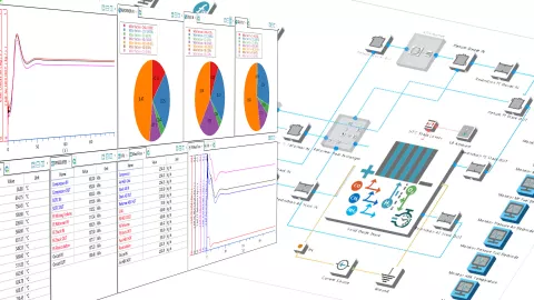
In Figure 3, the results of such a calibration are evident. For this specific low-temperature PEM fuel cell example, three operating points corresponding to the parameters, ionic conductivity, reference exchange current density on the cathode and through-plane tortuosity, were defined. The parameters are successfully adapted simultaneously to reach all three operating points.
A novel calibration algorithm has been integrated into FIRE M, specifically for fuel cells and electrolyzer cells. This innovative approach enables the calibration of a complete polarization curve by concurrently calculating various operating points. The approach is designed for real-life examples with large mesh sizes and limited calculation time while emphasizing ease of use. In summary, this calibration algorithm combines accuracy, efficiency, and user-friendliness—a valuable addition to the FIRE M toolkit.
Learn More About This Topic
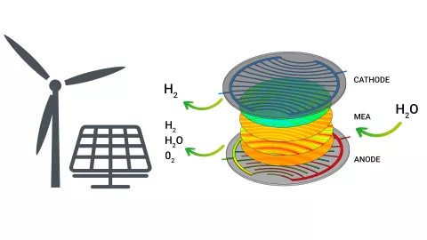
The demand for sustainably generated energy is increasing rapidly, and electrolyzers are seen as a promising technology. Due to their efficiency and good dynamic performance, PEM electrolyzers are one of the most widely used technologies today.
Aiming at a drastic CO₂ reduction in industry and mobility, the world is currently facing the challenge of producing green hydrogen at affordable prices and in sufficient quantities.

Electrolyzers – the technology at the heart of green hydrogen production – are currently in the focus of intense research and innovation activities, aiming at increased efficiency, minimized performance loss over time, and reducing development effort and time to market.